| Number | Figure | Caption | |
|---|---|---|---|
| 1 |  |
Two Gaussian distributions with unit width, with µ = 0.0 and µ = 0.5 in (a) and (b) respectively. We highlight the events in regions A (−∞, −1.5), B (−1.5, 0), C (0, 1.5), and D (1.5, ∞). |
|
 |
|||
| 2 | 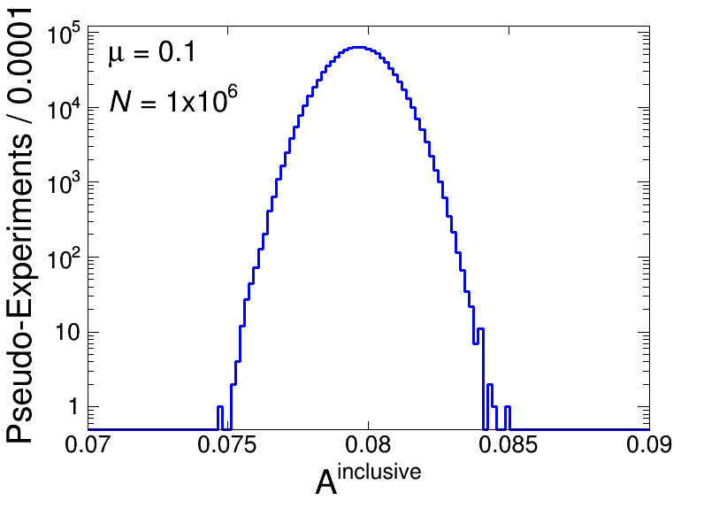 |
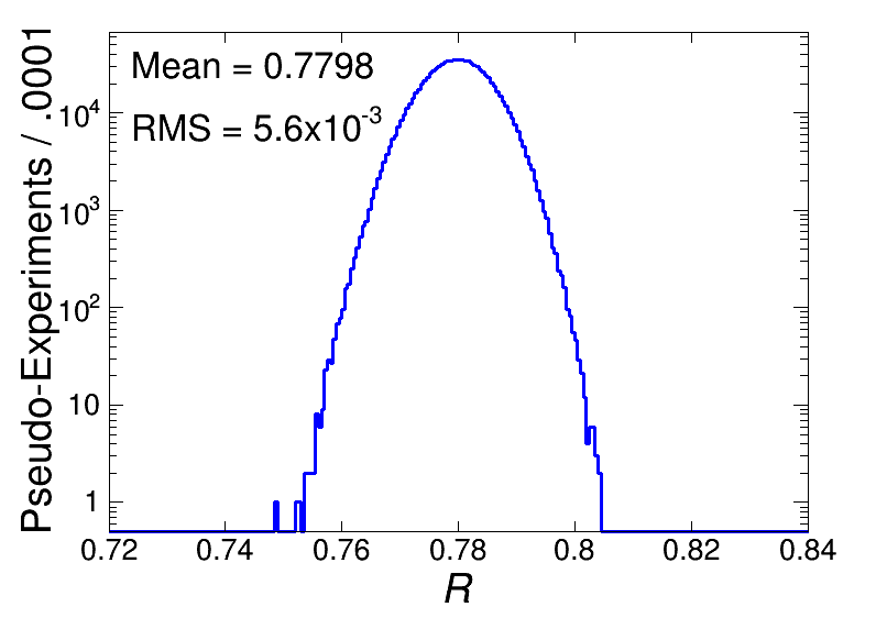
Distributions of Ainclusive, Avisible, and R in (a), (b), and (c) respectively. Each distribution has NPE=106 with N=106 and μ=0.1. |
|
 |
|||
 |
|||
| 3 |  |
Distributions of R with NPE=106 and μ=0.1, for N=105 and N=103 in (a) and (b) respectively. As N decreases, the estimation of R becomes worse; therefore obtaining the correct result with a single PE becomes statistically unreliable, the systematic uncertainty becomes both significantly large and asymmetric. Note the different x-axis scales in both plots. |
|
 |
|||
| 4 |  |
The same set of plots as in Fig. 3, but for μ=10−3 with N=109 and N=107 in (a) and (b) respectively. We note that the distribution transition also occurs for this μ, but at a larger value of N. |
|
 |
|||
| 5 | 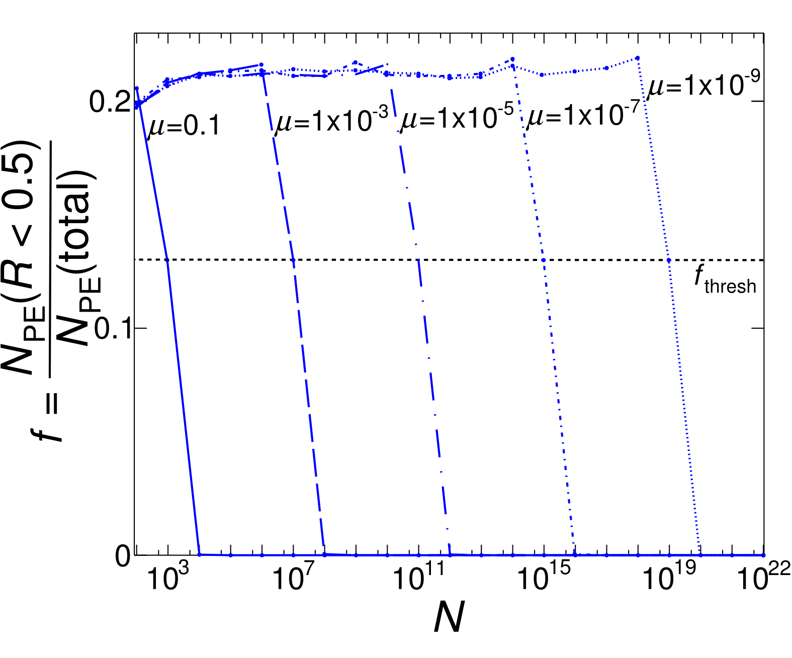 |
A plot showing |
|
| 6 |  |
A plot of Nthresh versus μ. Note that as μ→0, Nthresh approaches infinity. |
|
| 7 |  |
Distributions of R with NPE=106, for various small values of μ. In each case we have selected N large enough such that we are in the high statistics regime to ensure a reliable estimation of R, and we see that R converges to 0.7795 in all cases with small uncertainty. |
|
 |
|||
 |
|||
| 8 |  |
Contour plots of Avisible vs. Ainclusive for NPE=106 and μ=0.02. We have set N=104 and N=106 in (a) and (b) respectively. |
|
 |
|||
| A9 |  |
A plot of R determined analytically as a function of μ. We can see here how in the limit of small μ, R=0.7795 and only rises by 0.04% when μ=0.1. |
|